I use Kalman Filter to forecast next-day electricity price in France and Belgium, with the exogenous variables being the next-day load forecast and the next-day generation forecast. The France’s and Belgium’s electricity market are both in the European Power Exchange and intertwined.
The problem formulation of Kalman Filter is in the previous post.
Power Market Electricity Price Dataset
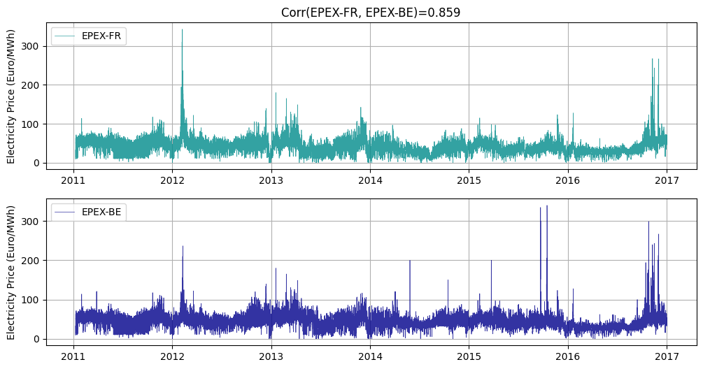
I found the dataset from this paper [1]. It contains hourly electricity prices in the EPEX-BE and EPEX-FR market, the day-ahead electricity market in Belgium and France, from 09 Jan, 2011 to 31 Dec, 2016. The price dataset contains 52416 rows with negative and zero prices as well as price spikes. Removing outliers when the electricity price is over 350 Euros per MWh or below 0, there’re 52367 ovservations. (I tried keeping these entries, but the Kalman Filter parameter estimates are “twisted” by these data points for a nontrivial period.) Prices in the two markets have a positive correlation of 0.859, which suggests there might be relative value trading opportunities.
Task 1: Mean-reverting Trading between France’s and Belgium’s Electricity Price
Problem Formulation
Following the Kalman Filter problem setup in my previous post, the idea is to formulate a State Space Model, with Belgium’s electricity price as observations \(Y_t = \text{EPEX-BE}_t\), France’s electricity price as the observation process \(H_t = \begin{bmatrix}1 & \text{EPEX-FR}_t \end{bmatrix}\) and the relationship between the two prices being hidden states \(X_t = \begin{bmatrix} \alpha_t & \beta_t \end{bmatrix}^T\).
\begin{align} Y_t= \text{EPEX-BE}_t & = \alpha_t + \beta_t \cdot \text{EPEX-FR}_t+\epsilon_t \\ &= H_t X_t + \epsilon_t, \epsilon_t \sim N(0, R_t) \end{align}
The hidden factors evolve in this way:
\begin{align} X_{t+1} & = \begin{bmatrix} \alpha_{t+1} & \beta_{t+1}]\end{bmatrix}^T \\ & = X_t + \eta_t, \eta_t \sim N(0, Q_t) \end{align}
Signal & Monetization
The choice of measurement error covariance \(R_t\) and process error covariance \(Q_t\), especially the ratio of values, matter a lot. Had we gathered data from physical observations, say with a motion sensor or a stopwatch, we can use the precision of instrument. For financial data, we can only estimate infer correlations and covariances from historical data or dynamics from domain knowledge. With some trial and error, I found a suitable covariance \(Q_t = Q\) independent of time (which can be revisted too).
Initial guesses also matter, but not as much as the covariances, since the Bayesian algorithm will constantly update the estimates. Given an initial guess, the Kalman Filter algorithm updates the estimated \(\alpha_t \beta_t\) as each observation comes in. The graph below shows the estimated \(\alpha_t \beta_t\), with the Mean Absolute Error of the Kalman Filter predictions being 1.566. Meanwhile, a baseline MAE of using today’s electricity price as next-day predicted price is 4.197. This suggests France’s EPEX electricity price indeed has some predictive powers for Belgium’s day-ahead EPEX electricity price.

We can try monetizing the relative value between France’s and Belgium’s electricity prices with a mean-reverting strategy. Denote \(\hat{Y}_t = H_t X_t\) as the predicted Belgium electricity price, \(Y_{err} = Y_t - \hat{Y}_t\), the goal is to find an interval of \(Y_{err}\) values for entry signal \([p_1,p_2]\), an exit level \(p_{\text{exit}}\), and a stop loss level \(p_{\text{stoploss}}\), with \(p_{\text{exit}} \le p_1 \le p_2 \le p_{\text{stoploss}}\). With a long or short signal, the position is \(\text{sign}\cdot \left (\text{EPEX-FR}_t - \beta_t \cdot \text{EPEX-BE}_t \right)\). For this project, I didn’t focus on the strategy, but created an interactive Python tool to back-test different price levels. The graph below on the left is the signals based on \(Y_{err}\). The graph below on the right shows a strategy with Sharpe ratio of 0.58.

Task 2: Use France’s Day-Ahead Generation Forecast to Predict France’s and Belgium’s Day-Ahead Electricity Price
Task 1 does not consider any exogenous variables besides the price data. This task tries to incorporate more information to the Kalman Filter.
Feature Engineering & Formulation
The paper [1] suggests the day-ahead grid load forecast and day-ahead generation forecast in France are the best predictors for both France’s and Belgium’s day-ahead electricity from current literature. This is possibly because of the increasing level of European electricity market integration and the two countries’ capacity. According to the 2016 IEA Energy Policies Review of France and Belgium [2][3], France had an estimated total suppy of 91.8 TWh renewable energy while Belgium had a total supply of 13.5 TWh. The feature selection process is worth revisting but I will use these variables for now.
The two features, day-ahead grid load forecast and day-ahead generation forecast in France, are available at the website of RTE, France’s Transmission System Operator. They exhibit cyclical patterns on levels of years, weeks, and days. The two features also have a high correlation of 0.908 over the period 2011-2016.
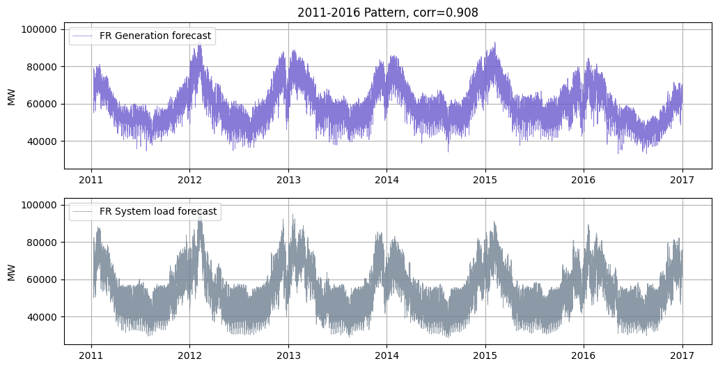
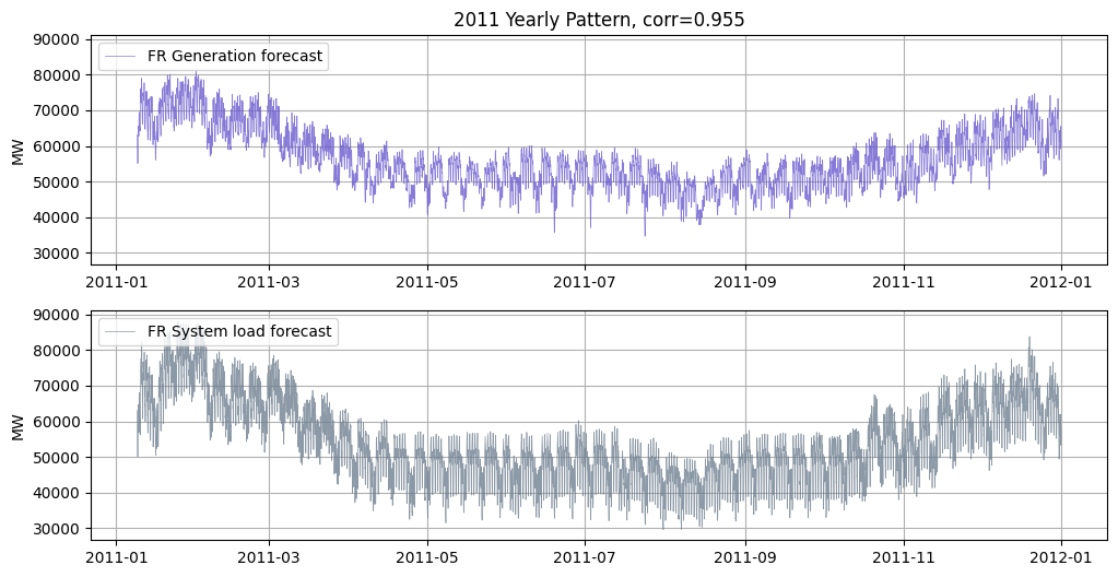
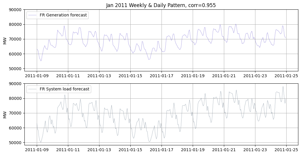
The France’s day-ahead load and generation forecasts are highly correlated, with a positive correlation of 0.9. If both are added as Kalman Filter states, the inverse of covariance matrices might sometimes be unexpectedly large. The two variables are also of the same physical unit (MW), so I decided to use the difference between them as a new feature, i.e., \(\text{load-gen-diff}_t = \text{load}_t - \text{generation}_t\). This new variable also makes sense as an excessive supply.
In this task, I decided to incorporate the information of two variables, France’s electricitiy price and difference between load and generation forecasts, to predict Belgium’s day-ahead electricity price. The problem setup can be revised to as follows: Belgium’s electricity price as observations \(Y_t = \text{EPEX-BE}_t\), France’s electricity price and load-generation difference as the observation process \(H_t = \begin{bmatrix}1 & \text{EPEX-FR}_t & \text{load-gen-diff}_t\end{bmatrix}\) and the relationship between the them being hidden states \(X_t = \begin{bmatrix} \alpha_t & \beta_{1,t} & \beta_{2,t} \end{bmatrix}^T\).
\begin{align} Y_t= \text{EPEX-BE}_t & = \alpha_t + \beta_{1,t} \cdot \text{EPEX-FR}_t+ \beta_{2,t} \cdot \text{load-gen-diff}_t + \epsilon_t \\ &= H_t X_t + \epsilon_t, \epsilon_t \sim N(0, R_t) \end{align}
The hidden factors evolve in this way:
\begin{align} X_{t+1} & = \begin{bmatrix} \alpha_{t+1} & \beta_{1,t+1} & \beta_{2,t+1}\end{bmatrix}^T \\ & = X_t + \eta_t, \eta_t \sim N(0, Q_t) \end{align}
Since the two features are of very different magnitutes, I used MinMaxScaler in sklearn.preprocessing to normalize the data by scaling each column linearly. I found normalization achieves better results than standardization via StandardScaler and RobustScaler. I think StandardScaler is not appropriate as there are outliers and the features do not follow normal distributions, whereas RobustScaler scales by quartiles and is better than StandardScaler, yet it’s is still not an appropriate non-linear scaling.
Signal & Monetization
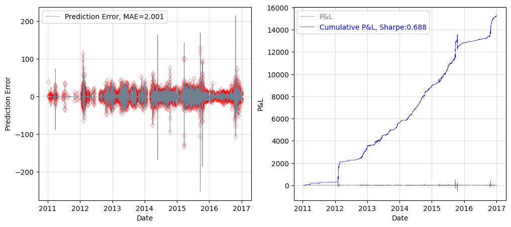
In this case, we can try monetizing the relative value with a momentum strategy. The graph below shows the prediction errors with the Mean Absolute Error of the Kalman Filter predictions being 2.001, and the red markers being signal points. Meanwhile, a baseline MAE of using today’s electricity price as next-day predicted price is 4.197. I didn’t spend too much time on the strategy, but used the interactive Python tool to back-test different price levels and entry/exit signal levels. The graph below shows a strategy with Sharpe ratio of 0.69.
References
-
Jesus Lago, Grzegorz Marcjasz, Bart De Schutter, Rafał Weron, Forecasting day-ahead electricity prices: A review of state-of-the-art algorithms, best practices and an open-access benchmark, Applied Energy, Volume 293, 2021, 116983, ISSN 0306-2619, https://doi.org/10.1016/j.apenergy.2021.116983.
-
Energy Policies of IEA Countries: France 2016 Review. https://www.iea.org/reports/energy-policies-of-iea-countries-france-2016-review.
-
Energy Policies of IEA Countries: Belgium 2016 Review. https://www.iea.org/reports/energy-policies-of-iea-countries-belgium-2016-review.