Kalman Filter on Simulated GPS Data

Kalman filter is a Bayesian method to update and improve parameter estimates from observations with uncertainty. It can be applied to time series formulated as a Linear Gaussian State Space Model. The kalman filter method was used by NASA in the Apollo Project to estimate trajectories of the manned spacecraft landing on the Moon and back (wow!).

In this and the next post, I will apply Kalman filter to two time series datasets: (1) simulated GPS locations (in honour of the Apollo 11 Lunar Module), and (2) a power market electricity price dataset.

Problem Formulation

Assumption: all noises are Gaussian, in which case the Kalman filter minimises the mean square error of estimated parameters. If the noises are not Gaussian, given only the mean and standard deviation, the Kalman filter is the best linear estimator.

The State Space Model, with observations $Y_t$ and hidden states $X_t$:

$$\begin{array}{rl}{Y}_t& =H_t{X}_t+{ϵ}_t,{ϵ}_t\sim N(0,R_t)\\ X_{t+1}& =A_t{X}_t+{\eta }_t,{\eta }_t\sim N(0,Q_t)\end{array}$$

where $R_t$ is the measurement error covariance matrix and $Q_t$ is the process error covariance matrix.

Using conclusions from the marginal and conditional distributions of multivariate Gaussians, and let $X_{t+1|t}$ be the predicted latent state with predicted mean ${\mu }_{t+1|t}$ and predicted covariance ${\mathrm{\Sigma }}_{t+1|t}$, the Kalman filter algorithm:

• At time 0, initial guess is $X_0\sim ({\mu }_{0|0},{\mathrm{\Sigma }}_{0|0})$
• At time t,
  • Prediction updates:

  $$\begin{array}{rl}{\mu }_{t+1|t}& =A_t{\mu }_{t|t}\\ {\mathrm{\Sigma }}_{t+1|t}& =A_t{\mathrm{\Sigma }}_{t|t}{A}_t^T+Q_t\end{array}$$

  • Measurement updates:

  $$\begin{array}{rl}{K}_{t+1}& ={\mathrm{\Sigma }}_{t+1|t}{H}_{t+1}^T{(H_{t+1}{\mathrm{\Sigma }}_{t+1|t}{H}_{t+1}^T+R_{t+1})}^{-1},\text{ the Kalman gain}\\ {\mu }_{t+1|t+1}& ={\mu }_{t+1|t}+K_{t+1}(Y_{t+1}-H_{t+1}{\mu }_{t+1|t})\\ & =(I-K_{t+1}{H}_{t+1}){\mu }_{t+1|t}+K_{t+1}{Y}_{t+1},\text{ the Innovation}\\ {\mathrm{\Sigma }}_{t+1|t+1}& =(I-K_{t+1}{H}_{t+1}){\mathrm{\Sigma }}_{t+1|t}\end{array}$$

Simulated Race Car Location Data

Suppose a race car is on a track with the following equations:

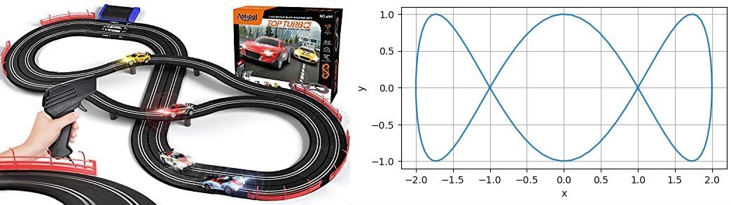
Suppose unfortunately the car jerks when accelerating (such that the acceleration is not constant), we consider the third order derivatives of the car’s position as Gaussian variables $a_x\sim N(0,{\sigma }_x^2),a_y\sim N(0,{\sigma }_y^2)$.

By the Newton’s law of motion,

$$\begin{array}{rl}x(t+\delta t)& =x(t)+\delta t\cdot \dot{x}(t)+\frac{\delta t^2}{2}\ddot{x}(t)+\frac{\delta t^3}{6}{a}_x\\ \dot{x}(t+\delta t)& =\dot{x}(t)+\delta t\cdot \ddot{x}(t)+\frac{\delta t^2}{2}{a}_x\\ \ddot{x}(t+\delta t)& =\ddot{x}(t)+\delta t\cdot a_x\end{array}$$

The dynamics are similar for dimension $y$.

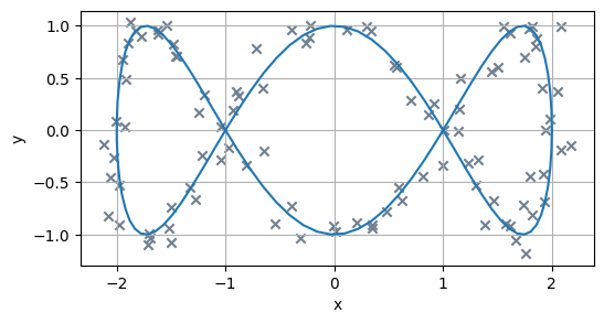
Let the car carry a GPS device to observe its current physical position, with measurement error following $ϵ\sim N(0,{\sigma }_{GPS}^2)$ on both dimensions. The observations might look like this:

Applying Newton dynamics to Kalman Filter, the state and observation vectors contain up to second order derivatives of the position (note $x,y$ are position on the 2D plane, and $X,Y$ are the hidden state and observation of the car’s GPS position):

$$\begin{array}{rl}X& ={\left[\begin{array}{cccccc}x& \dot{x}& \ddot{x}& y& \dot{y}& \ddot{y}\end{array}\right]}^T\\ Y& ={\left[\begin{array}{cc}{x}_{obs}& y_{obs}\end{array}\right]}^T\end{array}$$ $$A_t=\left[\begin{array}{cccccc}1& \delta t& \frac{\delta t^2}{2}& 0& 0& 0\\ 0& 1& \delta t& 0& 0& 0\\ 0& 0& 1& 0& 0& 0\\ 0& 0& 0& 1& \delta t& \frac{\delta t^2}{2}\\ 0& 0& 0& 0& 1& \delta t\\ 0& 0& 0& 0& 0& 1\end{array}\right]$$

The process error matrix covariance $Q$ is

$$\begin{array}{rl}Q& =Var({\left[\begin{array}{cccccc}\frac{\delta t^3}{6}{a}_x& \frac{\delta t^2}{2}{a}_x& \delta t\cdot a_x& \frac{\delta t^3}{6}{a}_y& \frac{\delta t^2}{2}{a}_y& \delta t\cdot a_y\end{array}\right]}^T)\\ & ={\sigma }_x^{2}u{u}^T+{\sigma }_y^{2}v{v}^T\end{array}$$

where $u={\left[\begin{array}{cccccc}\frac{\delta t^3}{6}{a}_x& \frac{\delta t^2}{2}{a}_x& \delta t\cdot a_x& 0& 0& 0\end{array}\right]}^T,v={\left[\begin{array}{cccccc}0& 0& 0& \frac{\delta t^3}{6}{a}_y& \frac{\delta t^2}{2}{a}_y& \delta t\cdot a_y\end{array}\right]}^T$

The GPS observes hidden states directly, so

$$H=\left[\begin{array}{cccccc}1& 0& 0& 0& 0& 0\\ 0& 0& 0& 1& 0& 0\end{array}\right]$$

and the measurement error covariance matrix $R$ is

$$R=\left[\begin{array}{cc}{\sigma }_{GPS}^2& 0\\ 0& {\sigma }_{GPS}^2\end{array}\right]$$

At time 0, suppose the car starts at the rightmost race track location (2,0) with known velocity and acceleration, and the hidden state covariance is a relatively large value due to uncertainty.

$$\begin{array}{rl}{X}_0& ={\left[\begin{array}{cccccc}2& 0& 2& 0& 3& 0\end{array}\right]}^T\\ {\mathrm{\Sigma }}_0& =0.5I_{6\times 6}\end{array}$$

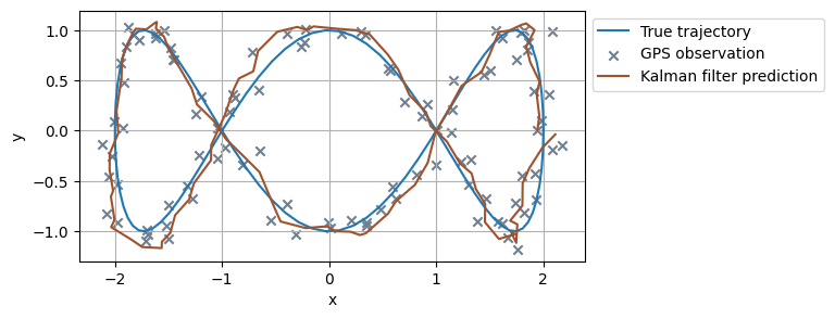
Here’re the results. The Kalman Filter algorithm updates the car’s predicted position as each observation comes in, which effectiveliy reduces noises and smoothes the raw GPS observations.