by Florent IDARGO & Sherry He

Hello !

This post is here to familiarize you with the structure of our data and its code usage, to have an easier readibility of it try to consult our github directory.

Recap

The FLASS project has for attempt to give traders insight about market reaction to YouTube trailers, from its nature it cannot be a long-term signal. We focused our analysis on 7 cinema studios (21 Century Fox, Disney, Lions Gate Pictures, Paramount Pictures, Sony Pictures, Universal Studio and Warner Bros), they all share a high movie release rate. Thus, we only expect to predict small movements in stock price as fundamentally, one movie does not account for a large revenue for these studios. Such movement is also expected to be short lasting as a constant news influx and high volatility in the stock market will dissolve the influence of our insights.

Objectives

Structure YouTube and Bloomberg Data in one file to run sicket-learn machine learning models.

Thus we got the following sub-objectives:
• Getting the right comments for the corresponding timeframe
• Building sentiment analysis measure on the corresponding comments
• Joining both financial and text data output in one file
• Fitting the right machine learning models, trying to find the performant hyperparameters through large combination test.

And the following hyperparameters to optimize: A: the comment selection period
B: the price variation prediction period

Worklow Detailing

1. Stored Data:

The raw data are stored in two main folders, for YouTube Comments they are kept in “Raw_Data_Studios” and Financial_Data”. for Financial data. Movies are linked to their studios financial data by their TICKER. For instance, the comments from the movie “Iron Man 2” are stored in a subfolder called “DIS” (Disney’s ticker) in the “Raw_Data_Studio” directory. Thus, each studio has its subfolder to segment the movies per studio, the data is therefore easily readable and can be manually retrieve while we can link movies to their financial data through their directory name.

2. The right comments:

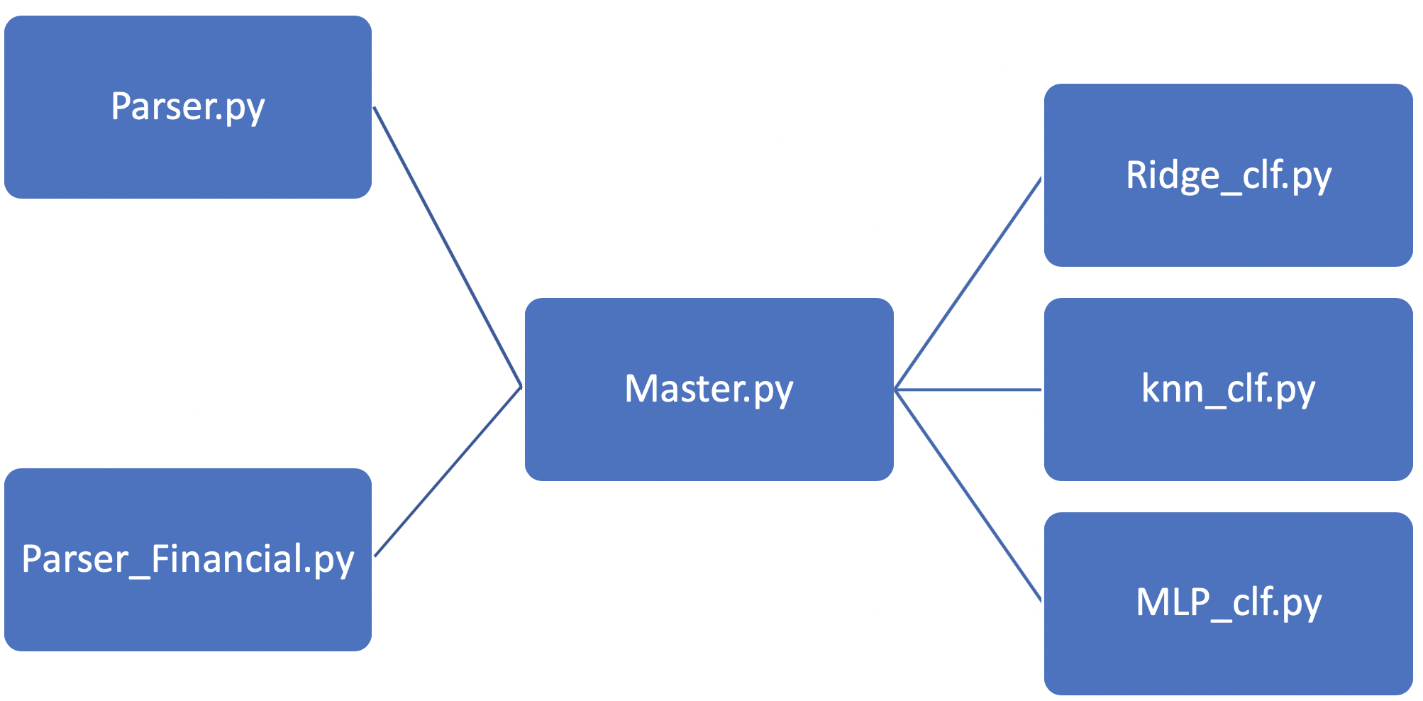
The comments have to be selected to correspond the chosen selection period and their text must be parsed to output a sentiment analysis signal. Such operation is handled in “working/Parser.py”, the main goal of this code is to go through the raw data files imported from YouTube (in “Raw_Data_Studios/NameOfTheTrailer_comments.csv”) through .json format.
For a given trailer, the Parser.py code will iterate through the comments first checking whether the given comment does correspond to the comment selection period. If it does, it will then execute TextBlob modules .polarity() and .subjectivity() functions to record each comments polarity. Finally, Parser.py output this result in a DataFrame, if the DataFrame does not record a minimum length of 5 comments over the chosen period of comment selection it won’t be return. Otherwise, the data is stored in the csv format in a dedicated file within the “Data_Studios/Movie’sStudioTICKER” directory.

3. Join the Data:

Once all studios have their movies’ comments interpreted with an assign polarity and subjectivity value stored, we structure them in a file joining this data and financial through “master.py”.
The purpose is to structure each of the movies as an individual input for later machine learning processes. Thus, for each movie we assign from Parser.py csv output its average comments polarity, subjectivity and the standard deviation of both characteristics to see their homogeneity.
Data extracted from comments:

As said before movies folder permit to retrieve their studio’s ticker and videos published time permit to select pertinent financial data. To help our model having financial context on each movies, we gave it the average volume and price variation over the 31 previous days as well as the standard deviation computed on the same time period. Finally, as we will run machine learning model, we need target columns, these will be called “Period_price_variation” and “Categorized_price_variation”. The first corresponds to the stock price evolution after the trailer’s release and the latter to a categorized version of this evolution. It would be 1 if the stock perform more than 2%, 0 if had stagnated and -1 if it decrease by more than 2% during the period.

4. Model testing:

Finally when having the necessary data structured in a DataFame all that remains is running sklearn machine learning models through several combination to obtain a satisfyingly performant model.
The model we chose are the Multilayer Perceptron Classifier, the K-nearest neighbor classifier and the Ridge Regression. For each of these models we needed to find the right combination of hyperparameter A and B in addition to the own models hyperparameters setting (i.e. layer structure setting, alpha, number of neighbor), this led to variable number of model testing. Whereas we tested 6’900 Ridge Regression models in total (69 combination of A&B were chose and for each we tested 100 values of alpha comprised in [0;1]), we had to do 69000 thousands test to achieve the same panel of analysis for MLP classifier (69 combinations of A&B and 1000 possible within (1,1,1) and (100,100,100)). As neuronal network is a highly time-consuming model to fit for sicket learn we decided to us KNN as a proxy, though it does absolutely not work in the same manner, as both models works with categorized output we expected to discern latent correlation in the data to thereafter analyze deeper with neuronal network. This process saved us 42’000 model fitting.

Final Workflow

Parser and Parser_Financial select the Data, Master join it in a common DataFrame and finally Ridge, knn and MLP models are runned in their respective files to test large combination set of hyperparameters.

Results

We were expecting to see the best results in the neuronal network MLP classifier, due to its really long processing time (it took us more than 24 hours to have our result file from MLP classifier), high complexity. The global enthusiasm concerning neuronal network had also biased us to see it as a “magical way” to get easy performance through large combination testing.
However, it seemed that our calibration of the model has failed to carry us further in performance than around 75% of accuracy on test data. This is quite deceptive for us but it is however a great leap forward to invest ourselves in the comprehension of such models architecture and notions.
KNN classifier did not provide any satisfying results neither, with fewer combination testing we had mainly took it as first indicator of latent data relationship on precise combination of A and B to test neuronal network model in a second step to optimize its running time. However, it has been the only model out of the three with high dispersion of A and B combinations. This made us dig through most combinations of A and B though we saved 75% of computing time by testing only 27’000 combinations out of 69’000.
With some distance, a better solution to save computing time from the three layers neuronal network parameters iteration would have been to compute over the whole model a 2 layers model with more limited parameters [from (1,1) to (50,50)]. This persistence of weight system through this heuristic would permits a better consistency between models and to better examine latent correlation between sentiment and stock price variation in the data.

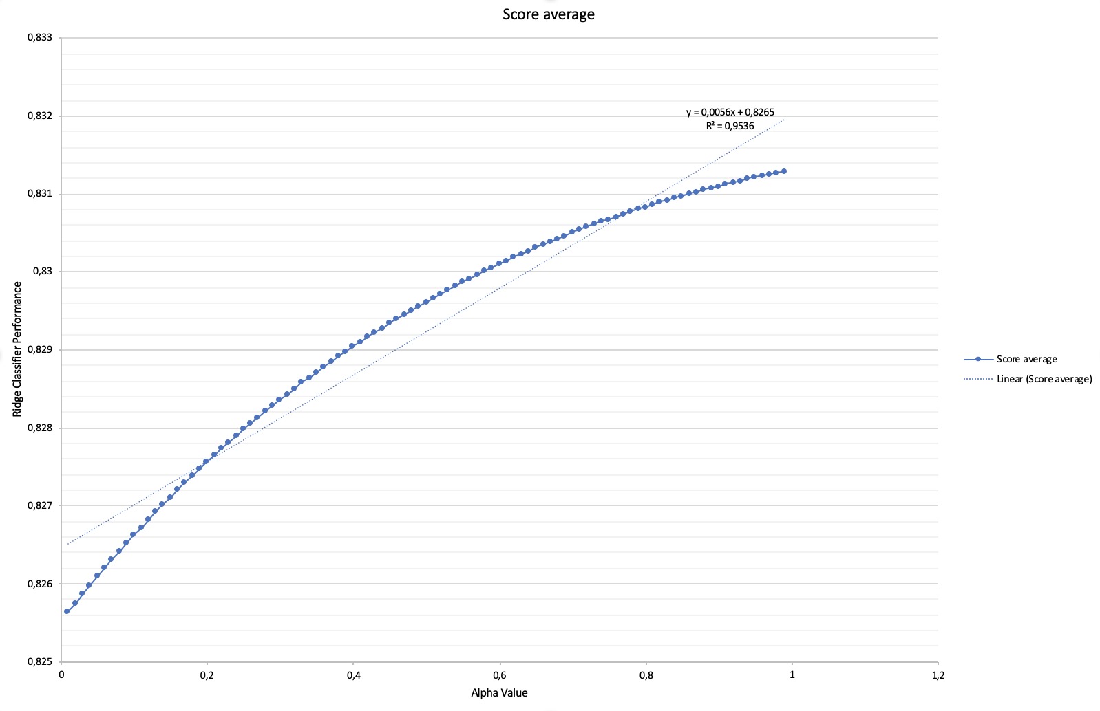
Finally, the Ridge regression machine learning model has been our best performing model, though most of its satisfyingly performant regressions were concentrated in (A,B = 1) it has permitted with low standard deviation (less than 5%) to observe a significant correlation between YouTube movies’ trailers sentiments and StockPrice. Causality is a much more complicated relationship to prove however the repeated performance of Ridge regression over Alpha values and close combination of A and B have built confidence in our stock price prediction model.



The top 200 results present relatively similar homogeneous combinations of price prediction period and comment selection period, however by 201 the results give favor to a longer calibration of A & B. After 239 the results are not anymore ordered and a variety of combinations are represented.

Thanks for having took lecture of our project, we had a great time learning from various fields in this project and are greatly pleased to finally have a great output.
Keep in touch with us and see you soon in other projects!👋🏽